With the growing demand for real-time applications, running deep learning models in the browser has become more accessible and powerful. In this post, we’ll explore how to implement object detection directly in the browser using YOLO (You Only Look Once) and TensorFlow.js. We will focus specifically on using a custom-trained YOLOv8 model for detecting human faces. By the end of this guide, you’ll learn how to set up and run the YOLO model for face detection using the TensorFlow.js library, process the results, and optimize its performance—all without needing a server or backend processing.
Why Run Neural Networks in the Browser?
Running neural networks in the browser offers several advantages:
- Low Latency: Everything happens client-side, avoiding the delay of sending data to a server and waiting for a response.
- Enhanced Privacy: Sensitive data remains on the user’s device, reducing the risk of breaches or exposure.
- Offline Capabilities: Users can access machine learning functionalities without a continuous internet connection.
- Cross-Platform Compatibility: Your application can run on any device with a browser—desktop, tablet, or smartphone.
Choosing and Preparing Your Neural Network
When selecting a neural network for browser implementation, consider factors like model size, speed, memory usage, and compatibility with browser technologies such as WebGL. For optimal performance on resource-limited hardware, it’s recommended to use models smaller than 30MB. Suitable models include MobileNetV2, SqueezeNet, EfficientNet, and certain YOLO variants. In our case, we opted for a custom-trained YOLOv8 model for detecting human faces in images.
If your model exceeds the recommended size, consider optimization techniques like quantization and pruning. Quantization reduces the precision of the model’s weights, typically converting 32-bit floating-point values to 16-bit or 8-bit integers. Pruning removes redundant connections in the neural network. Both methods shrink the model and reduce computational complexity, enhancing inference speed—especially on devices like smartphones—though they may slightly affect accuracy.
Optimizing YOLOv8 for Face Detection: Results from Our Custom Model
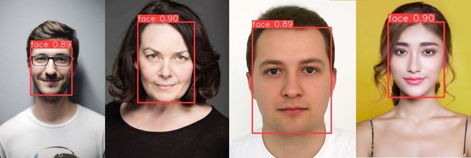
Our model is a YOLOv8 model trained on custom dataset to streamline document workflows. The goal was to automatically verify whether an attachment contains a clear, front-facing human photo, with no obstructions like masks. This is crucial for processes like ID verification, where the visibility of the person’s face is essential. Our dataset consisted of 1,500 images, split into 1,200 for training and 300 for validation. This allowed the model to learn how to distinguish between acceptable and unacceptable photos, ensuring accuracy in real-world use cases. The following images demonstrate how the network functions in practice.
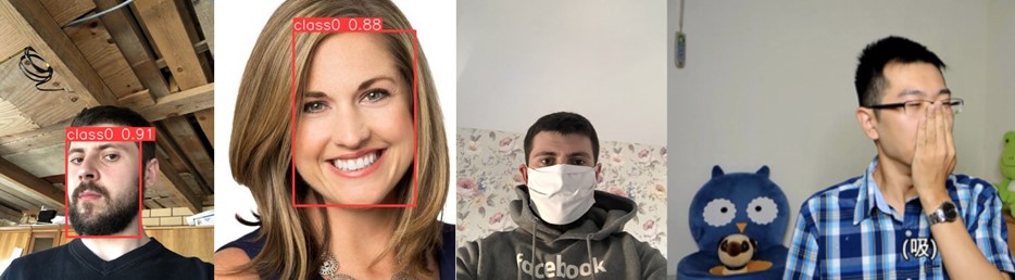
(source of images: https://www.kaggle.com/datasets/ashwingupta3012/human-faces, https://www.kaggle.com/datasets/andrewmvd/face-mask-detection)
Inference results on four examples – the two faces on the left were detected correctly, while the two on the right were not, as they were partially covered.
As a baseline for our model we selected YOLOv8s (small), which resulted in a model size of 44 MB and achieved 99.9% precision and 99.1% recall on our custom validation dataset. To explore model optimizations, we also tested a smaller baseline model, YOLOv8n (nano), and examined the effects of model quantization. Training with the YOLOv8n baseline produced a model sized at just 12 MB, with nearly identical accuracy metrics (99.7% precision and 99.1% recall). Next, we performed quantization on both models, the resultant model size and accuracy is shown in the table below:
| Baseline model | 16-bit quantized model | ||||
Size | Precision | Recall | Size | Precision | Recall | |
YOLOv8 small | 44 MB | 0.999 | 0.991 | 22 MB | 0.997 | 0.991 |
YOLOv8 nano | 12 MB | 0.997 | 0.991 | 6 MB | 0.989 | 0.991 |
Note: Recall measures how many actual positive samples were correctly identified, while precision indicates how many predicted positives were truly positive. For ideal case, they both are equal to 1.
In our example, using a smaller baseline model with quantization reduced accuracy by less than 1%, while shrinking the model size from 44 MB to just 6 MB.
Below are several example photos that illustrate how two networks: YOLOv8s and YOLOv8n with quantization operate:
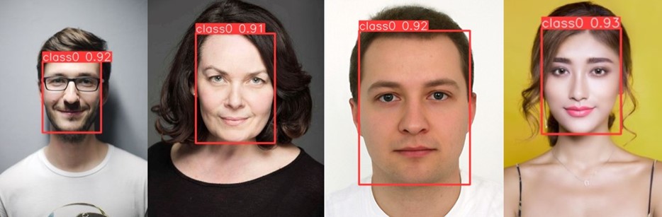
The results of inference with YOLOv8s model, without quantization (of size 44 MB). (source of images: https://www.kaggle.com/datasets/ashwingupta3012/human-faces).
| Loading model | Single inference | ||||
CPU 1 | CPU 2 | CPU 3 | CPU 1 | CPU 2 | CPU 3 | |
YOLOv8 small | 1050 ms | 3700 ms | 4200 ms | 21 ms | 117.5 ms | 196.5 ms |
YOLOv8 nano 16-bit | 980 ms | 3200 ms | 3700 ms | 16 ms | 112.5 ms | 189 ms |
Time improvement | 6.7 % | 13.5 % | 11.9 % | 23.8 % | 4.2 % | 3.8 % |
The results of inference with YOLOv8n model, with 16-bit quantization (of size 6 MB). There is only slight difference in confidence level, while location of bounding boxes is the same.
We tested the performance of two models—YOLOv8 small (44 MB) and YOLOv8 nano 16 bit quantized (6 MB)—across three different CPUs. The smaller model, YOLOv8 nano, consistently outperformed its larger counterpart in terms of both loading times and inference speed. Detailed performance metrics, including CPU-based loading and inference times, are summarized in the table above.
In addition to the CPU-based loading and inference times, another key factor to consider is the time required to download the models, which is not included in the table. Download times are directly proportional to the model size and are heavily influenced by the user’s network speed.
Getting Started: Setting up TensorFlow.js
To deploy your machine learning model in the browser, we’ll use TensorFlow.js, a powerful library that allows you to run pre-trained models or train new ones entirely in the browser. In this guide, we’ll focus on deploying a pre-trained YOLOv8 model for face detection. Below is a step-by-step guide to get TensorFlow.js set up and running.
1. Install TensorFlow.js
If you’re using a JavaScript bundler like Webpack or Parcel, you can install TensorFlow.js via npm:
npm install @tensorflow/tfjs
2. Load the Model
Since we’re using the TensorFlow.js library, you need to convert your model to the TensorFlow.js (Tf.js) format. In case of YOLO models, Ultralytics provides an easy way to achieve this with a simple command:
yolo export model=path/to/best.pt format=tfjs
Once converted, your model will be saved as binary files along with a JSON file called model.json. These files can be loaded into your application using the tf.loadGraphModel() function. Here’s an example of how to load the model, including warming it up with dummy input for performance:
export async function loadModel(modelPath) {
  try {
    // Load the model using a URL
    const model = await tf.loadGraphModel(`${modelPath}/model.json`);
    // Warm up the model
    const dummyInput = tf.ones(model.inputs[0].shape);
    await model.execute(dummyInput);
    return model;
  } catch (error) {
    throw new Error(`Failed to load model: ${error.message}`);
  }
}
3. Prepare the Input
Before running the model, we need to preprocess the input image. YOLO models expect images of a specific size, and ensuring that the input meets these requirements is crucial. Instead of merely resizing the image, we recommend a more sophisticated preprocessing method that maintains the aspect ratio and applies letterbox padding. This approach is consistent with the preprocessing used by Ultralytics during the training of the YOLO model.
The function below resizes, pads, and normalizes the input image to match the model’s required input size:
function preprocessImage(base64Image, imgSize) {
  const image = new Image();
  image.src = base64Image;
  const canvas = document.createElement('canvas');
  canvas.width = image.width;
  canvas.height = image.height;
  const ctx = canvas.getContext('2d');
  ctx.drawImage(image, 0, 0, image.width, image.height);

  // Convert canvas image to a tensor
  let imgTensor = tf.browser.fromPixels(canvas);

  // Determine rescale factor
  const xFactor = image.width / imgSize;
  const yFactor = image.height / imgSize;
  const factor = Math.max(xFactor, yFactor);
  const newWidth = Math.round(image.width / factor);
  const newHeight = Math.round(image.height / factor);

  // Resize to expected input shape
  imgTensor = tf.image.resizeBilinear(imgTensor, [newHeight, newWidth]);

  // Add padding
  const xPad = (imgSize - newWidth) / 2;
  const yPad = (imgSize - newHeight) / 2;
  const top = Math.floor(yPad);
  const bottom = Math.ceil(yPad);
  const left = Math.floor(xPad);
  const right = Math.ceil(xPad);
  imgTensor = tf.pad(imgTensor, [[top, bottom], [left, right], [0, 0]], 114);

  // Normalize pixel values
  imgTensor = imgTensor.div(255.0).expandDims(0); // Add batch dimension
  return { imgTensor, left, top, factor };

}
4. Run Inference
With the model loaded and the input preprocessed, we can now run inference to detect faces in the image:
const prediction = await model.execute(inputTensor);
5. Postprocess the Model Output
The YOLO network output is a tensor that needs to be properly interpreted. Below are the steps in our postprocessInferenceResults() function to extract the coordinates of all bounding boxes, classes, and confidence scores:
const results = prediction.transpose([0, 2, 1]);
const numClass = 1; // Only one class in our case
const boxes = tf.tidy(() => {
const w = results.slice([0, 0, 2], [-1, -1, 1]); // Get width
const h = results.slice([0, 0, 3], [-1, -1, 1]); // Get height
const x1 = tf.sub(results.slice([0, 0, 0], [-1, -1, 1]), tf.div(w, 2)); // Get x1

const y1 = tf.sub(results.slice([0, 0, 1], [-1, -1, 1]), tf.div(h, 2)); // Get y1
return tf.concat([y1, x1, y1.add(h), x1.add(w)], 2).squeeze();
});
To extract classes and confidence scores:
const numClass = labels.length;
const [scores, classes] = tf.tidy(() => {
const rawData = results.slice([0, 0, 4], [-1, -1, numClass]).squeeze(0);
  return [rawData.max(1), rawData.argMax(1)];
});
Next, filter out detections with confidence scores below a threshold (0.4) and overlapping bounding boxes:
const array = await scores.array();
const highConfidenceIndices = array.reduce((acc, value, index) => {
  if (value > 0.4) acc.push(index);
  return acc;
}, []);

const highConfidenceBoxes = boxes.gather(highConfidenceIndices);
const highConfidenceScores = scores.gather(highConfidenceIndices);
const highConfidenceClasses = classes.gather(highConfidenceIndices);
Finally, apply Non-Max Suppression (NMS) to filter out overlapping bounding boxes:
const nms = await tf.image.nonMaxSuppressionAsync(highConfidenceBoxes, highConfidenceScores, 40, 0.45, 0.4); // NMS to filter boxes

const boxesData = highConfidenceBoxes.gather(nms, 0); // Indexing boxes by NMS index
const scoresData = highConfidenceScores.gather(nms, 0).dataSync(); // Indexing scores by
const classesData = highConfidenceClasses.gather(nms, 0).dataSync(); // Indexing classes by NMS index
The last step is recalculating the coordinates to fit them into the shape of the original image:
// Precompute the margins and factors outside the stack
const yMarginTensor = tf.scalar(yMargin);
const xMarginTensor = tf.scalar(xMargin);
const resizeFactorTensor = tf.scalar(resizeFactor);
// Slice the boxesData and apply transformations in one step

const [yCoordinates, xCoordinates, height, width] =
  ['0', '1', '2', '3'].map((index) =>
    boxesData.slice([0, parseInt(index)], [-1, 1]).sub(index % 2 === 0 ? yMarginTensor : xMarginTensor).mul(resizeFactorTensor)
);

// Stack the tensors without converting to arrays (unless needed)
const bbox = tf.stack([yCoordinates, xCoordinates, height, width], 1);

// Convert to an array only if absolutely necessary
const bboxArray = bbox.arraySync();
At the end, we can define the runInference function, which summarizes the entire process of object detection. This function will handle image preprocessing, execute the model inference, and extract the resulting bounding boxes, confidence scores, and class labels. Here’s how it looks:
export async function runInference(model, labels, image, confidenceThreshold = 0.4) {
  try {
    // Preprocess the image
    const imgSize = model.inputs[0].shape[1];
    const { imgTensor: inputTensor, left: xMargin, top: yMargin, factor: resizeFactor } = preprocessImage(image, imgSize);

    // Run inference
    const prediction = await model.execute(inputTensor);

    // Post-process the model output
    const [boxes, scores, classes] = await postprocessInferenceResults(prediction, labels, xMargin, yMargin, resizeFactor, confidenceThreshold);
    return [boxes, scores, classes];

  } catch (error) {
    throw new Error(`Inference failed: ${error.message}`);
  }
}
6. Visualize the Results
Once we have our processed detections, it’s time to draw them on the canvas:
function drawBoxesOnCanvas(ctx, boxes, classes, scores, colors) {
  boxes.forEach((box, i) => {
    const [x1, y1, x2, y2] = box;
    ctx.strokeStyle = colors[classes[i]];
    ctx.lineWidth = 2;
    ctx.strokeRect(x1, y1, x2 - x1, y2 - y1);
    ctx.fillStyle = colors[classes[i]];
    ctx.fillText(`${labels[classes[i]]} (${Math.round(scores[i] * 100)}%)`, x1, y1);
  });
}
Running a YOLO model for object detection directly in the browser using TensorFlow.js opens up new possibilities for real-time applications. This guide covered everything from setting up TensorFlow.js to loading models, preprocessing images, running inference, and visualizing results. As you continue to explore this exciting technology, consider experimenting with different models, optimization techniques, and use cases to fully leverage the power of machine learning in web applications.